Getting to more than 1 Billion spin-flips per second on your laptop

Posted on December 12, 2024 by Jan Kaiser

There has been a lot of effort in simulating physics on computers. In the past, I have worked on accelerating magnetic systems like the Ising model on different computing hardware. For example, I have worked on simulating spins of a magnet on a Field Programmable Gate Array (FPGA). On an FPGA, emulators of magnetic spins can be laid out in space and it is relatively straight forward to update many spins per clock cycle as long as spin have only sparse connections. However, since FPGA clock frequencies are usually lower than that of CPUs, overall performance can not exceed around \(10^{12}\) spin flips per second (Ortega-Zamorano et al. 2016; Sutton et al. 2020). These FPGA designs are not general-purpose processors like conventional CPUs but are very specialized and usually take a long time to implement. They need to be designed with a specific FPGA in mind as well as needing to go through the synthesis, place & route and sign-off process. This is much more complex than a normal compiling step for compiling a conventional program written in Python or C++. General purpose graphics processing units (GPGPUs) have also been used to accelerate simulations of the 2D Ising model with comparable performance as for FPGAs (Romero et al. 2020).

In this blog post, we want to find out how fast we can run a 2D Ising model on a laptop. For a 2D Ising model, each spin as 4 neighbors. Some of this has been already done for more general Ising models by Isakov et al. (Isakov et al. 2015). Here, we are interested in the process of optimizing as well as finding a minimal implementation that does the trick. All codes can be found on Github.

Theoretical Background of the Ising Model

Why is the Ising Model an interesting problem to solve? The Ising model stands as a fundamental paradigm in statistical mechanics, offering insights into the behaviors of complex physical systems. Named after Ernst Ising, who fully solved the one-dimensional model in 1925, this mathematical framework provides a remarkably simple yet powerful representation of magnetic phase transitions and collective behavior in materials.

At its core, the Ising model represents a lattice of discrete magnetic moments, or spins, each capable of existing in one of two states: up (+1) or down (-1). These spins interact with their nearest neighbors through a coupling mechanism that captures the essential physics of ferromagnetic materials. The model’s simplicity belies its ability to capture complex phenomena such as phase transitions, critical behavior, and spontaneous symmetry breaking.

The fundamental Hamiltonian of the Ising model captures the system’s energy through the following expression:

\[H = -J \sum_{\langle i,j \rangle} \sigma_i \sigma_j - h \sum_i \sigma_i\]

where \(J\) represents the coupling strength between neighboring spins, \(\sigma_i\) represents the spin state at site \(i\) (either +1 or -1), \(h\) represents an external magnetic field, \(\langle i,j \rangle\) indicates summation over nearest neighbor pairs.

In the following sections, the code will be described on a high level. Each code is based on the one described in the previous section but will have added optimization. We will start with the most basic C++ implementation of simulating the 2D Ising model.

Basic Implementation

The basic version is using standard Markov Chain Monte Carlo Metropolis sampling. One spin is picked at random and updated serially as shown in the code snippet below. The difference in energy \(dE\) between spin being up or down depends on the state of the neighboring spins. In a Metropolis updating scheme, flips are accepted if energy is reduced. There is also a chance of accepting a flip if the energy increases where the energy is weighted by an exponential function.

void run_simulation() {
      std::vector<int> spins(N);
      std::random_device rd;
      std::mt19937 gen(rd());
      std::uniform_real_distribution<> dis(0.0, 1.0);
      
      auto update_start_time = std::chrono::high_resolution_clock::now();
      for (int step = 1; step <= steps; ++step) {
          for (int i = 0; i < N; ++i) {
              int x = std::uniform_int_distribution<>(0, L-1)(gen);
              int y = std::uniform_int_distribution<>(0, L-1)(gen);
              
              int dE = delta_energy(spins, x, y);
              if (dE <= 0 || dis(gen) < exp(-dE / T)) {
                  spins[x * L + y] *= -1;
              }
          }
      }
  }

Checkerboard updates

One major step in optimization is to partition the graph into groups of independent spins. For the 2D Ising model this can be done by partitioning the spins into two groups in a checkerboard pattern. Now all the white and all the black spins can be updated in parallel.

for (int step = 1; step <= steps; ++step) {
      // Update black and white sites separately
     update_spins(spins, 0, gen);  // Update black sites
     update_spins(spins, 1, gen);  // Update white sites
  }

This speeds up computation significantly by around 10x speed-up compared to the basic version.

Exponential lookup

Since the exponential function has to be computed many times while only 5 energy levels are possible with 4 neighbors, the exponential function can be pre-computed and looked up instead of calculated again every time. This gives us another 1.2x speed-up compared to the previous version (12x compared to baseline).

void initialize_exp_lookup(double T) {
      for (int dE = -MAX_DE; dE <= MAX_DE; ++dE) {
          exp_lookup[dE + MAX_DE] = exp(-dE / T);
      }
  }

Xorshiro Random Number Generator

Instead of using an expensive Mersenne Twister random number generator (RNG) algorithm, for our simple spin updates, we can use a much simpler pseudo RNG algorithm like Xorshiro. It is based on a linear feedback shift register with some additional bit rotations to make the RNG have more quality and make it less predictable. Overall, it speeds up the computation of the pseudo random number generation and the overall computation by 1.7x compared to the last version ( 20x compared to baseline).

Multithreading

Today’s laptops have multiple cores that allow for parallel execution through multithreading. However, data dependency and thread synchronization can also slow down a program. This is why it is important to make sure that data dependency between threads is limited. For example, we make sure that each Xorshiro RNG is run locally for each thread as shown below.

thread_local Xorshiro rng(std::random_device{}());

Multithreading with 14 threads gives us another relative speed-up of 4.5x compared to the Xorshiro RNG version and 90x total compared to baseline.

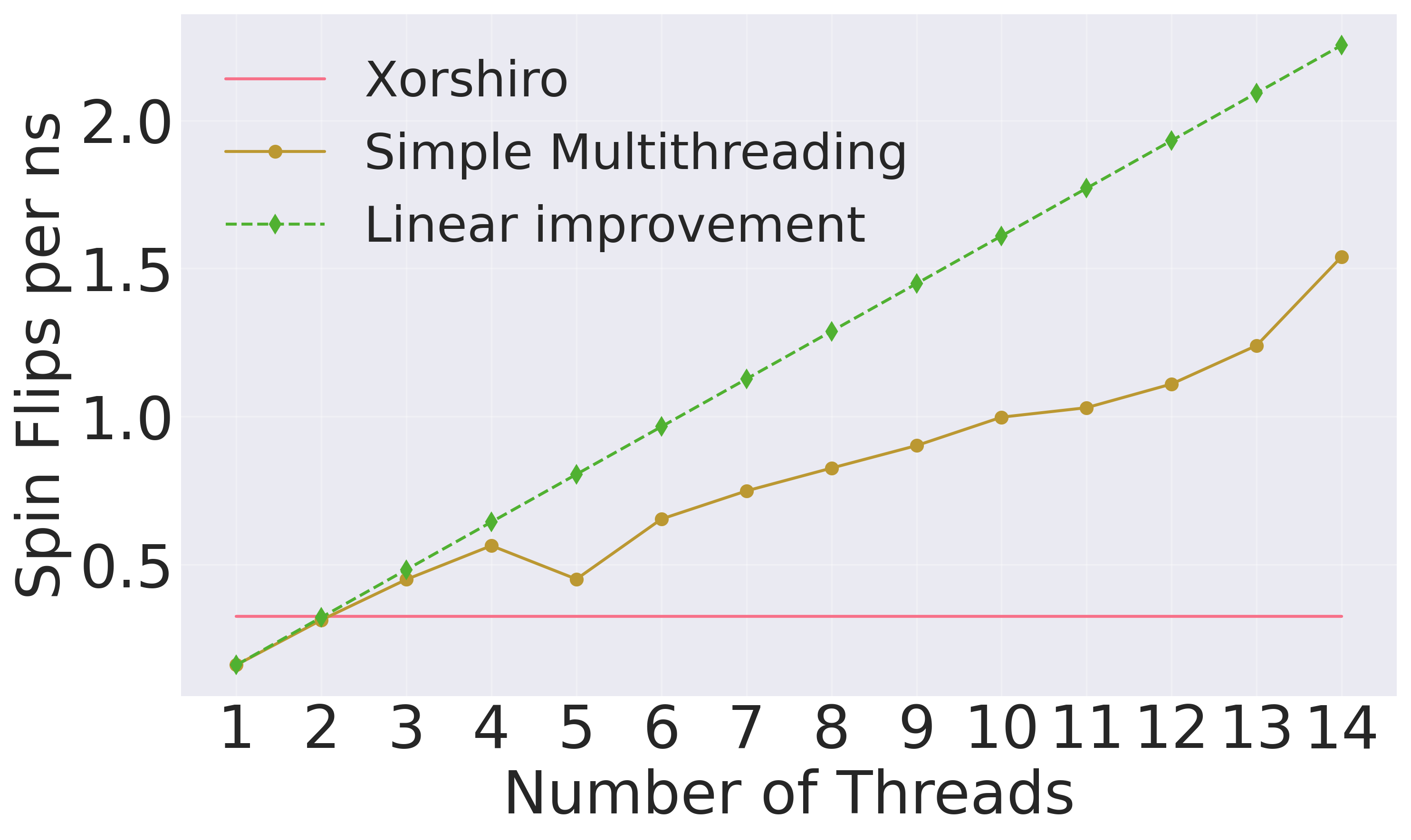
In Fig. 1, the spin flips per seconds are plotted versus number of threads. Note that initially for small number of threads, the performance is worse than the single threaded Xorshiro RNG code. For small number of threads, it can be seen that the performance almost goes up linearly (green line) for simple multithreading. After that the performance increase slows down when increasing the number of threads. However, we also do not see a clear plateau when using more threads. This means that in this massively parallel algorithm where we can update half of the spins in parallel, more parallelism like the ones GPUs can offer, can be very beneficial.

Multi-spin updates

The most advanced optimization on CPU that we will go over is one that is also done by Isakov et al. (Isakov et al. 2015). In the paper they run 64 simulations in parallel while storing the 64 spins from the identical site in an \(uint64\) data type. The energy calculation can be done with bitwise adding as shown below:

// Bitwise adding 
      uint64_t aligned_up = ~(center ^ up);
      uint64_t aligned_down = ~(center ^ down);
      uint64_t aligned_left = ~(center ^ left);
      uint64_t aligned_right = ~(center ^ right);
  
      uint64_t ud_sum = (aligned_up ^ aligned_down); //1st sum
      uint64_t ud_c = (aligned_up & aligned_down); //1st carry
  
      uint64_t lr_sum = (aligned_left ^ aligned_right); //1st sum
      uint64_t lr_c= (aligned_left & aligned_right); //2nd carry
  
      //add sums
      uint64_t b0 = (ud_sum ^ lr_sum); 
      uint64_t udlr_c = (ud_sum & lr_sum); //3rd carry
  
      //Full adder formula for carries
      uint64_t b1 = udlr_c ^ (ud_c ^ lr_c);
      uint64_t b2 = (ud_c & lr_c) | (lr_c & udlr_c) | (ud_c & udlr_c);

These bitwise operations make clever use of the CPU resources and hence boost the flips per seconds performance significantly giving us another 18x speed-up for total speed-up compared to baseline of around 1700x.

Utilizing GPUs with Apple Metal implementation

As a next step, we can use the built-in graphics processing capabilities. With Apple Silicon this can be done by utilizing Apple's Metal framework. For that we need to write the device code that will be run on the GPU and the host code that runs on CPU. The overall implementation looks very similar but we can now use the available 20 GPU cores to parallelize the application. This gives us a speed-up of 4x compared to the 14 Thread solution on CPU and around 385x compared to baseline. The code snippet below shows how one spin group is updated on the host side.

#include <Foundation/Foundation.hpp>
  #include <Metal/Metal.hpp>
  ...
  // Update black cells
  commandBuffer = commandQueue->commandBuffer();
  encoder = commandBuffer->computeCommandEncoder();
  encoder->setComputePipelineState(updatePipelineState);
              
  uint32_t color = 0;
  encoder->setBytes(&color, sizeof(color), 2);
  encoder->setBuffer(spinBuffer, 0, 0);
  encoder->setBuffer(paramsBuffer, 0, 1);
  encoder->dispatchThreads(gridSize, threadgroupSize);
              
  encoder->endEncoding();
  commandBuffer->commit();
  commandBuffer->waitUntilCompleted();
              
  // Update white cells
  ...

Multi-spin updates on GPU

As the final step we also want the test the multi-spin updates on GPU. Here, we rewrite the GPU kernel to do the same full adder additions that we described in section 7. This gives us around 5x speed-up compared to the multi-spin updates on GPU and  9070x speed-up compared to the CPU baseline. In the next section all results are summarized.

Benchmark Summary

Fig. 2 summarized the results with total run times running on an M4 Macbook Pro Chip. We have also added Isakov et al. (Isakov et al. 2015) spin per seconds running on the same machine. We are slightly better because the paper does not specialize the code to the 2D Ising model. The codes are available in (Kaiser 2024).

Conclusion

This optimization process showed that clever use of the laptop resources can lead to performance improvements of almost up to 4 orders of magnitude. Here, we have used both CPU multithreading and GPU programming with the Apple Metal Framework. All implementations are kept minimal and additional optimization especially for the GPU implementations should be possible.

References

If you found this post helpful, feel free to share it or reach out with questions.