During my PhD I worked on probabilistic computing and other hardware Monte Carlo methods and wanted to understand what different hardware can deliver on a well-defined workload. At some point, we looked at the simple benchmark of estimating π by sampling random points and spent some time optimizing it on a Field-Programmable Gate Array (FPGA). However, we did not put much effort into a Graphics Processing Unit (GPU) implementation, so the question we want to answer here is: how fast can a GPU actually go if you write proper CUDA C++?
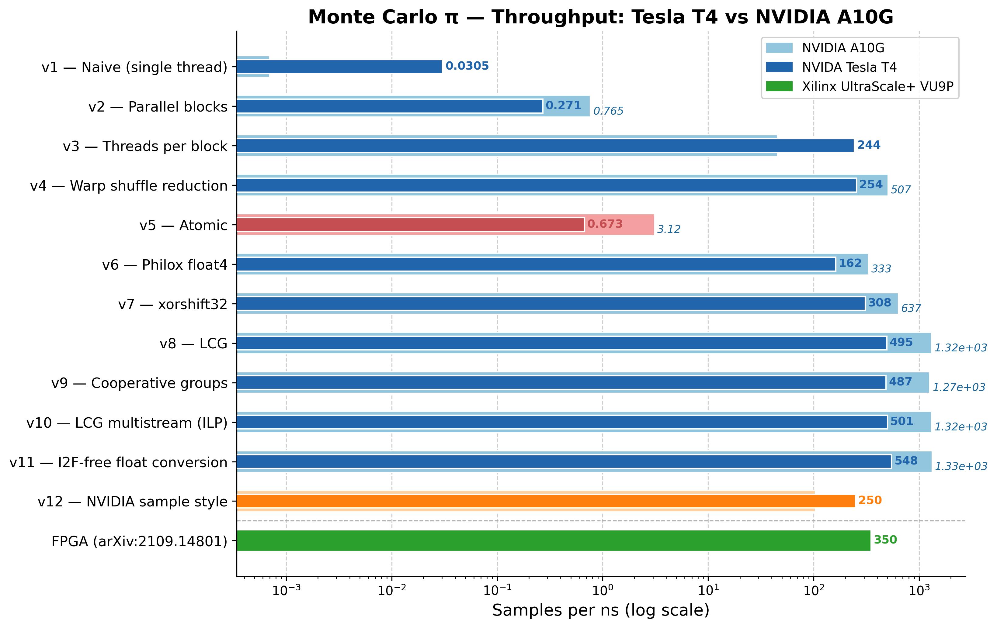
In this post we go through 12 CUDA versions, starting from a single-threaded kernel doing about 30 million samples per second and ending at around 550 billion samples per second on a NVIDIA Tesla T4 GPU, an 18,200× improvement over the baseline. All source code is on GitHub.
Theoretical Background
The idea is to draw $N$ random points uniformly in the unit square $[0,1]^2$ and count how many fall inside the quarter-circle $x^2 + y^2 \leq 1$. The fraction of hits converges to $\pi/4$,
$$\frac{N_{\text{hit}}}{N} \approx \frac{\pi}{4}$$and therefore:
$$\pi \approx 4 \cdot \frac{N_{\text{hit}}}{N}$$The error scales as $O(1/\sqrt{N})$, so around $10^{10}$ samples are needed for five reliable decimal places. Each sample is fully independent. First generate $x$ and $y$ then check $x^2 + y^2 \leq 1$ and accumulate the results. Hence, the problem maps directly onto the Single Instruction, Multiple Threads (SIMT) model of a GPU with no synchronization required during sampling.
Version 1 - Naive Single Thread
The baseline launches a single CUDA thread with picount<<<1,1>>>.
It uses curand's default XORWOW generator and runs 100,000 samples in a loop, leaving the
other ~2,500 CUDA cores on the T4 completely idle.
__global__ void picount(Count *totals, int seq_iter) {
    curandState_t rng;
    curand_init(clock64(), 0, 0, &rng);
    Count counter = 0;
    for (int i = 0; i < seq_iter; i++) {
        float x = curand_uniform(&rng);
        float y = curand_uniform(&rng);
        counter += 1 - int(x * x + y * y);
    }
    *totals = counter;
}
Throughput: 0.030 samples/ns.
Unsurprisingly, Nsight Compute (NCU) shows 0.33% compute throughput. A single block runs on one Streaming Multiprocessor (SM) while the other 39 sit idle. Within that block, one thread means 31 of 32 warp lanes are wasted. The top stall reason is a fixed-latency execution dependency from the XORWOW state-update chain. The fix is obvious: more threads.
Version 2 - Parallel Blocks
v2 launches one thread per block and uses the occupancy API to choose the number of blocks. Each block gets a unique seed offset:
int tid = blockIdx.x;
curand_init(clock64(), tid, 0, &rng);
The host sums the partial results after the kernel returns. Throughput: 0.27 samples/ns, a 9× improvement, but each block still uses only one of its 32–1024 available threads.
NCU tells a different story now: compute is at 86% and occupancy near 98%. The bottleneck has shifted from "not enough threads" to "pseudorandom number generator (PRNG) cost". curand's XORWOW generator needs 59 registers per thread, enough to fill the SM's 65,536-register file with a single 1024-thread block. Register pressure becomes the occupancy constraint for the rest of the curand-based versions.
Version 3 - Threads per Block + Shared Memory
v3 uses all threads in each block. Every thread accumulates into its own slot in a shared memory array, and thread 0 does a sequential reduction at the end:
extern __shared__ Count counter[];
int tid = threadIdx.x + blockIdx.x * blockDim.x;
curand_init(clock64(), tid, 0, &rng);
counter[threadIdx.x] = 0;

for (int i = 0; i < seq_iter; i++) {
    float x = curand_uniform(&rng);
    float y = curand_uniform(&rng);
    counter[threadIdx.x] += (x*x + y*y <= 1.0f) ? 1 : 0;
}
__syncthreads();
if (threadIdx.x == 0) {
    for (int i = 1; i < blockDim.x; i++)
        counter[0] += counter[i];
    totals[blockIdx.x] = counter[0];
}
Throughput: 244 samples/ns, a 900× jump over v2, simply from using all available threads.
NCU shows 86% compute at 100% occupancy —
essentially the same utilization as v2 despite the ~900× throughput gain.
The improvement is entirely from using all threads, not from doing the work
differently. One overhead worth noting: the shared memory counter[]
array gets read and written on every iteration, 100,000 times per thread.
Version 4 - Warp Shuffle Reduction
Instead of the sequential reduction by thread 0, we can use __shfl_down_sync
for a warp-level reduction. Threads in the same warp exchange register values directly
without touching shared memory:
Count val = counter[threadIdx.x];
for (int offset = WARP_SIZE/2; offset > 0; offset /= 2)
    val += __shfl_down_sync(0xffffffff, val, offset, WARP_SIZE);

__shared__ Count warp_totals[MAX_WARPS_PER_BLOCK];
if (lane == 0) warp_totals[warp_id] = val;
__syncthreads();

if (threadIdx.x == 0) {
    int num_warps = blockDim.x / WARP_SIZE;
    totals[blockIdx.x] = 0;
    for (int i = 0; i < num_warps; i++)
        totals[blockIdx.x] += warp_totals[i];
}
Throughput: 254 samples/ns, a 1.04× gain over v3. The reduction is no longer the bottleneck.
Not much changes in the profile: compute rises slightly to 88%
and registers stay at 63. The real difference is shared memory usage — v3
allocates 8 KB dynamically for the per-thread counter[]
array while v4 uses only 256 bytes for warp_totals[].
The modest gain comes from eliminating the sequential reduction loop where 1023
threads sat idle at __syncthreads(). Both versions are still
bottlenecked on the XORWOW ALU cost — the reduction was never the problem.
Version 5 - Atomic Accumulation
This version replaces the warp reduction with a single shared counter that all threads
update via atomicAdd:
__shared__ Count shared_counter;
if (threadIdx.x == 0) shared_counter = 0;
__syncthreads();

for (int i = 0; i < seq_iter; i++) {
    float x = curand_uniform(&rng);
    float y = curand_uniform(&rng);
    atomicAdd(&shared_counter, (x*x + y*y <= 1.0f) ? 1 : 0);
}
Throughput drops to 0.67 samples/ns, worse than v2. All 1024 threads serialize on the same address every single iteration. Atomics work well for infrequent updates, but not for this.
The NCU profile makes clear what is happening. L1/TEX throughput hits 99.72% while compute sits at only 49% and SM busy at 22%. Every cycle, 1024 threads fight over a single shared address. The L1 cache handles all the requests (nothing touches DRAM), but the serialization queue drains so slowly that the FP32 pipelines are starved for work. Not a bandwidth problem — a contention problem.
Version 6 - Philox float4 (4 Samples per RNG Call)
Philox is a counter-based generator that returns four 32-bit values at once.
Using curand_uniform4 and striding the loop by 4 gives four samples
per call:
curandStatePhilox4_32_10_t rng;
curand_init(clock64(), tid, 0, &rng);

for (int i = 0; i < seq_iter; i += 4) {
    float4 rands = curand_uniform4(&rng);
    counter[threadIdx.x] += (rands.x*rands.x + rands.y*rands.y <= 1.0f) ? 1 : 0;
    counter[threadIdx.x] += (rands.z*rands.z + rands.w*rands.w <= 1.0f) ? 1 : 0;
    // ... (two more from a second call)
}
Throughput: 162 samples/ns, which is actually slower than v4. Philox has good statistical quality but its per-output cost is higher than XORWOW. The 4× output per call does not compensate for the heavier state update. NCU shows compute at only 61.5% despite 100% occupancy — 33% of warp cycles are stalled waiting for the math pipeline. Philox's deeper instruction sequence overloads the execution pipes and the warp scheduler cannot hide the latency.
Version 7 - Custom xorshift32
Instead of curand, we write a simple xorshift32 directly in device code. xorshift32 is three XOR-shift operations with a period of $2^{32} - 1$:
__device__ unsigned int xorshift32(unsigned int *state) {
    unsigned int x = *state;
    x ^= x << 13;
    x ^= x >> 17;
    x ^= x << 5;
    *state = x;
    return x;
}

float x = xorshift32(&state) / (float)UINT_MAX;
float y = xorshift32(&state) / (float)UINT_MAX;
Throughput: 308 samples/ns, 1.9× faster than v6. The lightweight PRNG removes all the library overhead. NCU shows compute at 87.6% with the Arithmetic Logic Unit (ALU) pipeline as the top-utilized unit — no stalls, just useful arithmetic. The bottleneck is now the sampling math itself.
We note that the FPGA reference (Kaiser et al., 2021) also uses xorshift, so v7 is the most direct comparison between the two: same algorithm, different hardware.
Version 8 - LCG + Register Accumulator
A Linear Congruential Generator (LCG) is even simpler than xorshift32: one multiply and one add per output. It has known weaknesses (correlated high-order bits, hyperplane structure) but for a hit test, which only needs to distinguish "inside" from "outside", the bias is negligible at these sample counts.
The second change in v8 is accumulating into a plain register instead of shared
memory. Previous versions write to counter[threadIdx.x] on every
iteration, a shared memory read-modify-write 100,000 times per thread. With a
register instead:
__device__ unsigned int lcg(unsigned int *state) {
    *state = 1664525u * (*state) + 1013904223u;
    return *state;
}

Count local = 0;
for (int i = 0; i < seq_iter; i++) {
    float x = lcg(&state) / (float)UINT_MAX;
    float y = lcg(&state) / (float)UINT_MAX;
    local += (x*x + y*y <= 1.0f) ? 1 : 0;
}
// single shared memory write after the loop
Count val = local;
Throughput: 495 samples/ns, a 1.6× improvement over v7. The register change accounts for the whole gain.
NCU shows the kernel is now compute-bound at 98.9% SM utilization with memory effectively idle. There is an interesting subtlety in the pipeline breakdown: by elapsed cycles the Fused Multiply-Add (FMA) unit is highest at 77.3% (single-precision floating-point/FP32 arithmetic), but by executed instruction count the integer/special-function execution (XU) unit leads at 98.9%. XU handles integer operations including the LCG multiply, so the instruction mix is actually dominated by integer work, not floating-point.
The dominant warp stall (47% of cycles) is the Memory Input/Output (MIO) instruction queue being full. On Turing the MIO queue is the pathway for integer multiplies, and 200,000 of them per thread saturates it completely. Warp switching hides individual multiply latency but cannot drain a queue that is continuously full.
At this point the kernel is the only bottleneck — memory traffic is negligible. So where do we go from here? There are a few things worth trying: doing the final reduction on-device instead of the host, using instruction-level parallelism (ILP) to hide the LCG's serial dependency, and looking for unnecessary instructions feeding the MIO queue.
Version 9 - Cooperative Groups (On-device Final Reduction)
In all previous versions the host loops over per-block partial sums after the
kernel returns. That loop is not included in the kernel timing (the CUDA event
timer wraps only the kernel launch), so it does not affect the numbers in the
table. Still, moving the reduction on-device is worth showing as a technique.
The Cooperative Groups API lets us do it: after all blocks write their partial
sums, grid.sync() synchronizes the whole grid and block 0 does the
summation, so only a single scalar gets copied back:
#include <cooperative_groups.h>
namespace cg = cooperative_groups;

__global__ void picount(Count *totals, Count *grand_total, int seq_iter) {
    cg::grid_group grid = cg::this_grid();
    // ... sampling and block-level reduction into totals[blockIdx.x] ...

    grid.sync(); // grid-wide barrier

    if (blockIdx.x == 0 && threadIdx.x == 0) {
        Count sum = 0;
        for (int i = 0; i < (int)gridDim.x; i++)
            sum += totals[i];
        *grand_total = sum;
    }
}
The kernel must be launched via cudaLaunchCooperativeKernel, which
requires SM 6.0+ and the grid to fit in the GPU's resident capacity.
Throughput: 487 samples/ns, same as v8. The host-side
reduction was never in the timed path to begin with, so this is expected.
What v9 does show is that the grid.sync() barrier and on-device
reduction add negligible overhead to the kernel itself. This pattern matters
more for kernels where you actually need intermediate results to stay on the GPU.
Version 10 - LCG Multistream (Instruction-Level Parallelism)
The LCG has a serial dependency chain — each output depends on the previous one. A natural idea is to run multiple independent LCG streams per thread so the hardware can interleave them and hide the multiply latency. Here we use four streams:
// x-streams use one LCG family, y-streams use a different one
// to avoid cross-stream correlation (LCG hyperplane problem)
__device__ __forceinline__ unsigned int lcg_step(unsigned int s) {
    return 1664525u * s + 1013904223u;   // Numerical Recipes
}
__device__ __forceinline__ unsigned int lcg_step_y(unsigned int s) {
    return 1103515245u * s + 12345u;     // glibc / BSD
}

for (int i = 0; i < seq_iter / STREAMS; i++) {
    s0 = lcg_step(s0);   float x0 = s0 * scale;
    s1 = lcg_step_y(s1); float y0 = s1 * scale;
    s2 = lcg_step(s2);   float x1 = s2 * scale;
    s3 = lcg_step_y(s3); float y1 = s3 * scale;
    // ... second set of 4 advances ...
    local += (x0*x0 + y0*y0 <= 1.0f) ? 1 : 0;
    // ...
}Throughput: ~500 samples/ns, same as v8. The NCU profile tells us why: v10's MIO stall share is 48% — slightly worse than v8's 47%. Four independent LCG chains just feed four times as many integer multiplies into the same saturated MIO queue. The bottleneck is pipeline throughput, not instruction latency. Warp switching hides latency by moving to another warp while one waits, but that does not help when the issue queue itself is full. More chains only add more pressure.
So ILP is not the answer here. That leaves one more thing to look at: are there unnecessary MIO instructions inside the loop we can get rid of?
Version 11 - I2F-Free Float Conversion
It turns out there are two unnecessary MIO instructions per iteration. The LCG
multiply (1664525u * state) is unavoidable, but the I2F
(integer-to-float) conversions that turn the raw output into a float
are not. Even with a precomputed scale constant, the compiler still emits I2F —
it is a real instruction that takes up an MIO slot, twice per iteration
(once for each coordinate).
I2F can be eliminated by reinterpreting the LCG bits directly as an IEEE-754 float. A single-precision float stores a sign bit, 8 exponent bits, and 23 mantissa bits. Any value with exponent = 127 and sign = 0 lies in $[1.0, 2.0)$. Taking the top 23 bits of the LCG output and ORing them into that pattern gives a float in $[1.0, 2.0)$ with no conversion instruction at all:
__device__ __forceinline__ float uint_to_float01(unsigned int x) {
    // Top 23 bits → mantissa; exponent=127 → value in [1.0, 2.0).
    // __uint_as_float is a zero-cost bitwise reinterpret, no instruction emitted.
    return __uint_as_float((x >> 9) | 0x3f800000u) - 1.0f;
}

for (int i = 0; i < seq_iter; i++) {
    float x = uint_to_float01(lcg(&state));
    float y = uint_to_float01(lcg(&state));
    local += (__fmaf_rn(y, y, x * x) <= 1.0f) ? 1 : 0;
}Throughput: 548 samples/ns, a 1.1× improvement over v10. NCU duration drops from 22.1 ms to 20.0 ms, a solid 10.7% reduction. Compute throughput actually falls from 99% to 85.6%, which looks like a regression but is not — with two fewer MIO instructions per iteration the SM finishes the same work in fewer total cycles while being less continuously saturated.
The remaining bottleneck is the LCG multiply itself, the last MIO consumer in the loop. I tried replacing the LCG with xorshift32 (three dependent XOR-shift ops, no multiply) but it was slower: the three-instruction dependency chain costs more cycles than one multiply with partial stall hiding.
Version 12 - NVIDIA Sample Implementation
The NVIDIA CUDA Samples repository ships a
Monte Carlo π estimator
(MC_EstimatePiInlineP), filed under Concepts and Techniques.
It is a sample, written to demonstrate the curand API clearly rather than to maximise
throughput. To that end, v12 is a faithful single-file port compiled with exactly the same flags
(-O3 --use_fast_math) as every other version here.
Three structural differences from our tuned kernels are deliberately preserved:
- Global-memory curandState. Each thread allocates a 48-byte XORWOW
state in Dynamic Random-Access Memory (DRAM). A separate
initRNGkernel writes the states, thencomputeValueloads them back, two full DRAM round-trips before any sample is drawn. - Two kernel launches. The init and compute passes are separate kernels, adding a second kernel-launch overhead and defeating any chance of the compiler fusing the init into the hot loop.
- Shared-memory tree reduction. Each reduction level writes to
sdata[]and calls__syncthreads(), whereas v4+ use__shfl_down_sync, which stays entirely in registers within a warp.
v12 uses the same XORWOW generator as v1–v4, so comparing v12 to v3/v4 isolates the structural overhead (global-memory RNG state, two kernel launches, shared-memory tree reduction) with the PRNG held constant. Any gap between v12 and v8 is then separately explained by the LCG being faster than XORWOW regardless of code structure.
NCU puts numbers on each cost. The initRNG kernel alone takes
4.15 ms — it writes 48-byte XORWOW states to DRAM with a badly
strided access pattern where only 3.6 of every 32 bytes per cache sector are
used, wasting 89% of bandwidth. It also generates 140 divergent
branches per warp from curand's skip-ahead logic, whereas every other
version in this series has zero.
The computeValue kernel launches 400 blocks on 40 SMs, producing
2.5 waves. That fractional third wave accounts for up to 33%
of runtime, and occupancy drops to 84%. Rounding to 320 or 480 blocks would
fix this.
FPGA Reference Implementation
The FPGA result in the comparison chart comes from Kaiser et al. (2021), which implements Monte Carlo π estimation on a Xilinx UltraScale+ VU9P. The design is built around three components that map well onto FPGA resources.
Random number generation uses xorshift linear feedback shift registers (LFSRs). An LFSR is a purely combinational circuit made of flip-flops and XOR gates.
The hit test ($x^2 + y^2 \leq 1$) requires two multiplications and an addition.
DSP48 slices, the hard multiply-accumulate blocks in UltraScale+, perform
A*B + C natively in a single operation. One bank of 2,800 DSPs computes
$x^2$ and a second bank of 2,800 DSPs computes $y^2 + x^2$ in one step by feeding
$x^2$ into the C port, giving 5,600 DSPs total with no separate
adder needed. This produces 2,800 hit-test results per clock cycle.
Collecting 2,800 binary results into a single counter each cycle requires an adder tree. A balanced binary tree halves the partial sums at each level. Since $\lceil \log_2 2800 \rceil = 12$, the tree needs 11 pipeline stages to reduce 2,800 inputs to one sum. This can be fully pipelined so a new accumulated total of 2800 hit tests exits the adder tree every clock cycle.
At 350 samples/ns the FPGA beats the T4 at v7 (same xorshift algorithm, 308 samples/ns) but falls below the LCG variants on the T4, and well below the A10G numbers. The FPGA also requires full synthesis, place-and-route, and timing closure to build — considerably more involved than compiling CUDA C++.
Benchmark Summary
| Version | Key technique introduced | Samples/ns | Speed-up vs baseline |
|---|---|---|---|
| v1 - Naive | Single thread, curand XORWOW | 0.030 | 1× |
| v2 - Parallel blocks | One thread per block, occupancy API | 0.27 | 9× |
| v3 - Threads per block | Shared mem accumulator, sequential reduction | 244 | 8,000× |
| v4 - Warp reduction | __shfl_down_sync reduction | 254 | 8,350× |
| v5 - Atomic | atomicAdd demonstration | 0.67 | 22× |
| v6 - Philox float4 | 4 samples per curand call | 162 | 5,300× |
| v7 - xorshift32 | Custom device PRNG, drop curand | 308 | 10,100× |
| v8 - LCG + register | LCG, register accumulator | 495 | 16,300× |
| v9 - Cooperative groups | Grid-wide sync, on-device reduction | 487 | 16,000× |
| v10 - LCG multistream | 4 ILP streams, dual-family LCG pairing | 500 | 16,400× |
| v11 - I2F-free conversion | Bit-reinterpret float, eliminate I2F from MIO queue | 548 | 18,000× |
| v12 - NVIDIA sample style | Global curandState, 2 kernels, smem tree reduction | 250 | 8,200× |
| FPGA (Kaiser et al., 2021) | Dedicated FPGA logic (reference) | 350 | 11,500× |
The Compute Ceiling
Nsight Compute data on the Tesla T4 shows the progression across the final versions:
| Metric | v10 | v11 (I2F-free) |
|---|---|---|
| Compute (SM) Throughput | 99.4% | 85.6% |
| Memory Throughput | 0.01% | 0.01% |
| Achieved Occupancy | 100% | 100% |
| NCU Duration (ms) | 22.1 | 20.0 |
| Registers per Thread | 42 | 42 |
| Block limit (registers) | 1 block/SM | 1 block/SM |
The entire working set stays in registers throughout, so memory is effectively idle. Register pressure (42 × 1024 = 43,008 per SM) fills the 65,536-register budget and limits both versions to one block per SM, but that is enough for 100% occupancy.
The drop in compute throughput from 99.4% to 85.6% in v11 looks like a regression but is not. In v10 the MIO queue is continuously full, forcing frequent stalls. In v11 two I2F instructions per iteration are gone, the queue drains faster, and the SM finishes the same work in fewer cycles — it just looks less busy while doing so. Wall-clock time is what matters: 20.0 ms vs 22.1 ms. To push further from here you would need a different data type (half-precision floating-point/FP16 on tensor cores, at the cost of quantization bias), a different algorithm like quasi-Monte Carlo with Sobol sequences, or simply a faster GPU.
Hardware Upgrade: Tesla T4 vs NVIDIA A10G
Once the software is saturated, the next question is what a different GPU gives. We ran the same binaries on an Amazon Web Services (AWS) g5 instance (A10G) and a g4dn instance (T4):
| GPU | SMs | FP32 peak (TFLOPS) | v8 (samples/ns) | v9 (samples/ns) | v10 (samples/ns) | v11 (samples/ns) |
|---|---|---|---|---|---|---|
| NVIDIA Tesla T4 | 40 | 8.1 | 495 | 487 | 500 | 548 |
| NVIDIA A10G | 72 | 31.2 | 1,316 | 1,265 | 1,317 | 1,334 |
| A10G / T4 ratio | 2.66× | 2.60× | 2.63× | 2.43× | ||
The A10G is 2.63× faster on v10 with no code changes. Three hardware differences explain the gap: more SMs (72 vs 40, 1.8×), more CUDA cores per SM (Ampere GA102 has 128 FP32 cores per SM versus Turing's 64, thanks to a second datapath alongside the INT32 pipeline), and a higher boost clock (~1695 MHz vs ~1590 MHz, ~1.07×). Together these give a 3.85× FP32 peak ratio.
The measured 2.63× speedup is lower than the 3.85× peak because our kernel is bottlenecked on the integer MIO queue, not the FP32 pipes. Throughput scales more with SM count than with FP32 peak. This also explains why v10 and v11 perform identically on the A10G (12.03 ms vs 11.88 ms): on Turing, I2F and IMUL compete for the same MIO queue so removing I2F helps; on Ampere both route through a unified ALU pipeline where the bottleneck stays saturated either way.
A practical note on cost: the T4 on a g4dn instance is cheaper per hour than an AWS F1 FPGA instance. The A10G on g5 costs roughly 3-4× more than a g4dn, so the 2.63× speedup comes at a price.
Conclusion
The biggest single gain (~900× from v2 to v3) came just from using all available threads. No algorithmic cleverness is needed; filling the hardware is the first thing to do. After that, lighter primitives helped at each step: a custom xorshift beat curand's Philox, a simple LCG beat xorshift, and moving the accumulator from shared memory to a register gave another 1.6×. After v8 the kernel appeared saturated at 99.4% compute utilization, but NCU profiling showed the true bottleneck was MIO queue saturation from I2F conversion instructions, not FP32 throughput. Eliminating them via bit-reinterpretation (v11) gave a further 10.7% reduction in cycle count, reaching 548 samples/ns.
A useful reference point is the FPGA implementation from Kaiser et al. (2021), which runs at 350 samples/ns on a Xilinx UltraScale+ VU9P using an xorshift generator. That makes v7 the closest comparison: 308 samples/ns on the T4 and 637 samples/ns on the A10G. The T4 instance is also cheaper to rent than an AWS F1 FPGA instance, so the GPU is competitive on cost as well.
All codes are available at github.com/kaiser1711/Monte-Carlo-Pi-with-CUDA.
References
Kaiser, Jan. 2026. "Monte-Carlo-Pi-with-CUDA." GitHub. https://github.com/kaiser1711/Monte-Carlo-Pi-with-CUDA.
Kaiser, J., Jaiswal, R., Behin-Aein, B., & Datta, S. (2021). "Benchmarking a Probabilistic Coprocessor." arXiv:2109.14801 [cs.ET]. https://doi.org/10.48550/arXiv.2109.14801.
NVIDIA. "MC_EstimatePiInlineP — Monte Carlo Estimation of Pi (inline PRNG)." CUDA Samples. https://github.com/NVIDIA/cuda-samples/tree/master/Samples/2_Concepts_and_Techniques/MC_EstimatePiInlineP.
If you found this post helpful, feel free to share it or reach out with questions.